Contents
Introduction: The Frame is Not Part of Nature
Representations of Lie Groups and Lie Algebras
Rotation in 3 Dimensions and Angular Momentum
Rotation in 4 Dimensions and Relativistic Space-Time
Rotation in 2 Dimensions and Electromagnetism
Rotation in Field Spaces and Nuclear Forces
Appendices: Lie groups, Noether’s theorem, exterior calculus, Hodge dual, special relativity, and Riemannian geometry
Introduction: The Frame is Not Part of Nature

When I first learned about vectors in high school, vector addition made perfect sense. But the dot product puzzled me: why not just multiply component by component and get a vector result? When my math teacher introduced the cross product, I was perplexed: what a strange crisscross pattern! I wondered: can I make up other ways of multiplying two vectors together, maybe using a zigzag pattern?
To answer these questions, we need to talk about symmetry groups and their representations.
Here’s what’s going on: To describe physical reality with numbers (mathematically), we first need to set up a coordinate frame. Then, we can determine the coordinates of the relevant features. Coordinate frames, however, are not part of nature, they exist only in our imagination! Usually there is a large (often infinite) choice of possible frames, all equally good. But each frame leads to a different mathematical description of the same physical reality. Luckily, all these descriptions are related by coordinate transformations, which together form a symmetry group. For a mathematical model to make physical sense, it must take these symmetries into account! We say that it must be formulated in terms of quantities that furnish representations (or realizations) of the relevant symmetry group.
What does this mean when applied to vector geometry? To describe 3D geometrical objects mathematically we use the x, y, z coordinates of their centers, vertices, etc. But because space is isotropic, the necessary coordinate frame can be set up with an arbitrary orientation. The coordinate triplets, which result from all possible frames, are related by 3D rotation matrices. Together, these (infinitely many) rotation matrices form the Lie group SO(3). For a mathematical model to make geometrical sense, we formulate it in terms of quantities that furnish representations of SO(3). Such quantities are the scalars, vectors, and tensors. Moreover, operations acting on these quantities must again yield quantities of this type. Such operations are the dot product, the cross product, the tensor (or outer) product, and that’s pretty much it. Thus, while the component-wise and zigzag vector multiplications, alluded to above, are mathematically possible, they are geometrically meaningless!
In other words, it is the SO(3) symmetry of our space that gives rise to notions like the dot and cross products. Similarly, it is the SO+(1,3) symmetry of space-time that motivates the tensor notation with upstairs and downstairs indices and the associated products used in relativity. Finally, it is the U(n) symmetry of Hilbert space that motivates Dirac’s notation with “kets” and “bras” and the associated products used in quantum mechanics.
As we will see, the symmetries of Nature and the frame independence that they demand essentially determine what fields and particles can exist and what their dynamical laws are!
Symmetry groups also play an important role for Noether’s theorem, which makes a connection between continuous symmetries and conserved quantities in classical physics. Moreover, symmetry groups are central to quantum mechanics, where observables are associated with operators rather than simple variables. If such an operator has a discrete eigenvalue spectrum, quantized values are observed, and if two such operators do not commute, observations are limited by an uncertainty relation. These quantum-mechanical operators turn out to be (proportional to) generators of symmetry groups!
Finally, symmetry groups are at the heart of gauge theory, our best theory of the fundamental forces and interactions. Famously, the standard model of particle physics is based on the Lie group SU(3)xSU(2)xU(1). This group and its representations provide the key to understanding the electromagnetic force and the nuclear interactions at a fundamental level!
The following tutorial is structured like a series of mini adventures. Our journey takes us from classical and quantum mechanics to special relativity, to electrodynamics, and finally to nuclear physics. Representation theory will act as our guide! Each mini adventure comes in the form of a concrete example or application and is presented on a single sheet (two pages) with a diagram followed by an explanation. No prior knowledge of group or representation theory is required; however, a basic understanding of physics is expected (Susskind’s Theoretical Minimum, Vol. 1-3 or Schwichtenberg’s No-Nonsense series are good sources to get up to speed).
Here Is The Plan
- First, we familiarize ourselves with the main ideas of Lie groups, Lie algebras, and their representations. The details will be filled in in the subsequent examples.
- In examples 1.1 to 1.31, we explore rotation in 3-dimensional Euclidean space by examining the Lie groups SU(2), SO(3), and Sp(1). These examples illustrate many aspects of Lie theory in a setting that is familiar and intuitive to us. We’ll study angular momentum in its various forms: classical and quantum mechanical, orbital and intrinsic, entangled and unentangled. Finally, we discuss how quaternions are related to rotation.
- In examples 2.1 and 2.2, we explore reflection and the idea of parity by examining the discrete groups D3 and Z2.
- In examples 3.1 to 3.10, we explore rotation in 4-dimensional Euclidean space by examining the Lie groups SO(4) and Spin(4). After this warm-up exercise, we turn to 4-dimensional space-time according to the special theory of relativity. In examples 3.11 to 3.28, we explore Lorentz transformation of space-time by examining the Lie groups SO+(1,3), Spin+(1,3), and SL(2,C). Besides rotations (changes in orientation), we now also have boosts (changes in inertial motion). Understanding the representations of these groups clarifies what kind of fields and particles can exist in our space-time. We discover the dynamical laws governing these fields and particles, namely the Klein-Gordon, Weyl, Dirac, Maxwell, and Proca equations.
- In examples 4.1 to 4.13, we explore rotation in two dimensions by examining the Lie groups U(1) and SO(2). Applying these rotations to complex (quantum) fields that represent charged matter introduces us to gauge theory. After learning about local transformations and a little bit of differential geometry, we are rewarded with a deep understanding of electromagnetic interactions. Maxwell’s equations (describing how charges and currents produce EM fields) and the Lorentz force law (describing how charges and currents are pushed around by EM fields) naturally arise from symmetry constraints.
- In examples 5.1 to 5.5, we explore SU(2) gauge theory and its application to (quantum) fields that represent particle doublets. This exercise introduces us to the weak nuclear interactions, which are responsible for radioactive decay, supernova explosions, and more.
- Additional information about Lie groups, Noether’s theorem, exterior calculus, Hodge dual, special relativity, and Riemannian geometry can be found in the Appendices.
I hope you enjoy these mini adventures as much as I did! Of course, there are many more groups with important applications to physics, such as the Poincare group and SU(3), but that’s for another day.
Click on any of the diagrams to get an explanation!
Representations of Lie Groups and Lie Algebras

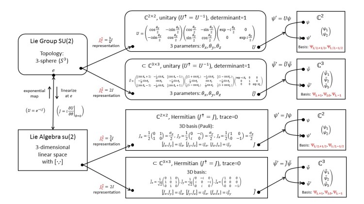
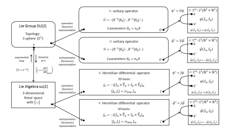
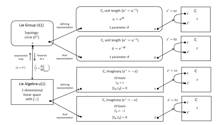
We begin with an overview of Lie groups, Lie algebras, and representation theory. The diagram shown below helps us to get oriented (click on it for a detailed explanation!).
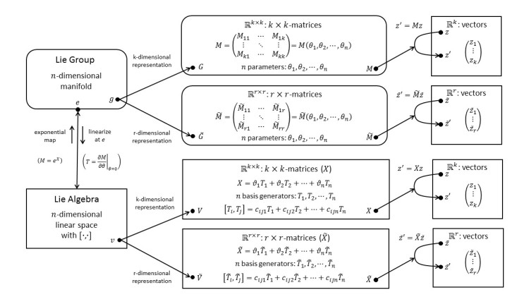
The basic idea behind a Lie group is to describe continuous symmetry transformations that depend on a couple of parameters. For example, all possible rotations of a 3D object parametrized by the rotation angles about the x, y, and z axes form a Lie group.
The basic idea behind a representation is to map abstract transformations to concrete matrices. For example, the group of all possible rotations of a 3D object can be mapped to the set of 3×3 rotation matrices. These matrices, in turn, act on vectors, which are the elements of the representation space. We say that these vectors furnish the representation of the group. In our example, the representation space consists of 3-component column vectors.
Interestingly, Lie groups do not have just one, but many (usually infinitely many) representation! We will see many examples of that.
The basic idea behind a Lie algebra is to provide a simplified (linearized) description of the Lie group by considering only small transformations. Surprisingly, almost no information is lost by going from the Lie group to the Lie algebra! As with the Lie group, the abstract Lie algebra can be made concrete by mapping it to a set of matrices. These matrices act on the same representation space as the matrices of the corresponding group representation.
We can always go from a Lie-group representation to the corresponding Lie-algebra representation by differentiating (linearizing) it. Going from the Lie algebra back to the Lie group by integrating it is a bit more tricky because there can be more than one group for the same algebra. This backwards path is known as the exponential map.
The above diagram will serve as a template for the specific examples that we are going to explore. We will fill specific groups, matrices, and vectors into the boxes.
Don’t worry if not everything is clear at this point. We will go through many examples that illustrate and clarify the theory. The idea is to learn by exploring examples! You may want to skim over the theory and come back for more details after you have gone through some of the examples.
Rotation in 3 Dimensions and Angular Momentum

SU(2)
1.1 SU(2): The Special Unitary Group of Degree Two

Let’s get started with the first example! The group SU(2) is perfect for that: it is rich enough to illustrate most features of Lie groups, yet simple enough to serve as an introductory example. Moreover, it is one of the most important groups in physics! Here, we learn about the 2-dimensional or defining representation of SU(2) and its associated Lie algebra su(2). Surprisingly, this group, which is defined in terms of 2×2 matrices, also has a 3-dimensional representation!
1.2 SU(2): Application to Quantum-Mechanical Spin

What is this good for? Unitary groups and their representations are tailor-made for quantum mechanics: The Lie-group representation tells us how quantum states transform and the Lie-algebra representation gives us the operators for the quantum observables. In particular, SU(2) is exactly what we need to describe spin. Here, we discuss spin-1/2 and spin-1 particles.
1.3 SU(2): Four- and Five-Dimensional Representations; Higher Spins

SU(2) has infinitely many representations. Here, we look a the 4- and 5-dimensional irreducible representations, which describe spin-3/2 and spin-2 particles, respectively. We discuss what quantum-mechanical spin really is.
1.4 SU(2): Defining Representation with Axis-Angle Parameters

Representations can be parametrized in many different ways, resulting in mathematical expressions that look very different from each other although they describe the same representation. Here, we look at the defining representation of SU(2) with axis-angle parameters.
1.5 SU(2): Defining Representation with 3-Sphere Parameters; Group Topology

We look at yet another parametrization of the same representations. This one reveals to us the topology of SU(2): a beautiful 3-sphere! We discuss several ways to visualize this elusive object.
1.6 SU(2): Trivial Representation; Invariants

The 1-dimensional or trivial representation maps everything to the identity element. What is this good for? It describes spin-0 particles and invariants, such as the action!
1.7 SU(2): Dual and Complex-Conjugate Representations; Similarity Transformations
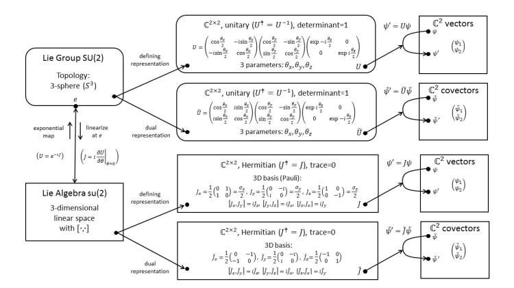
For every representation there is a dual representation, which acts on covectors instead of vectors. In the case of unitary representations, the dual representation is also the complex-conjugate representation. How is the defining representation of SU(2) related to its dual? We learn about similarity transformations.
1.8 SU(2): Adjoint Representation; Transforming the Generators
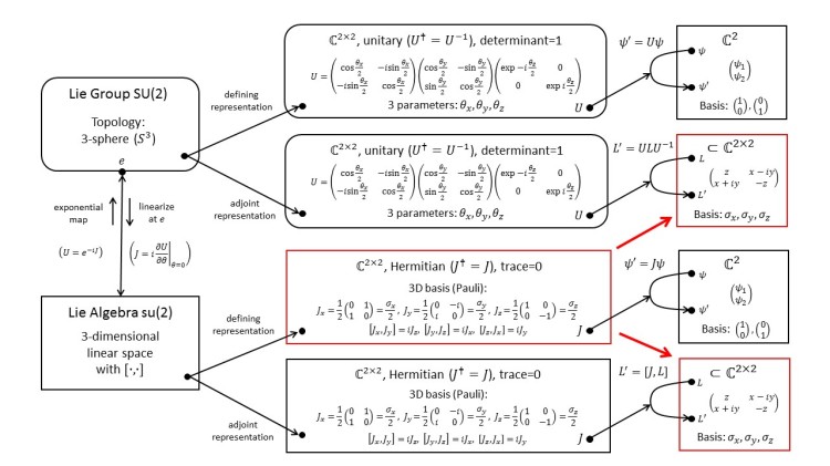
Every Lie group has a distinguished representation, called the adjoint representation, that tells us how the generators of the group transform. We learn that SU(2), which is defined in terms of complex matrices, also has a representation on real vectors! More about this in the next example.
1.9 SU(2): Representation on Real 3-Dimensional Vectors; Spinors vs. Vectors

After “unpacking” the adjoint representation, we are led to transformations that we know well: rotations of ordinary 3D vectors! We compare the mysterious spinors of the defining representation with the straightforward vectors of our new representation.
1.10 SU(2): Labels for Basis Vectors and Representations; Casimir Operator
Before tackling more complicated representations, we need to introduce some important concepts. We discuss how to construct a meaningful basis for the representation space and assign labels to the basis vectors. Then, we introduce the Casimir operator, which helps us to delineate irreducible representations.
SU(2) and Functions
1.11 SU(2): Infinite-Dimensional Representations; Functions and Differential Operators

We study an infinite-dimensional representation of SU(2) acting on a simple quantum-mechanical wave function. We become familiar with Lie algebras that have differential operators as their elements.
1.12 SU(2): Application to Orbital Angular Momentum; Spherical Harmonics

With the infinite-dimensional representation we have what it takes to understand the orbital angular momentum of a wave function. We learn about spherical harmonics, the states of definite angular momentum.
1.13 SU(2): Application to Electron Orbitals; Reducible Representations
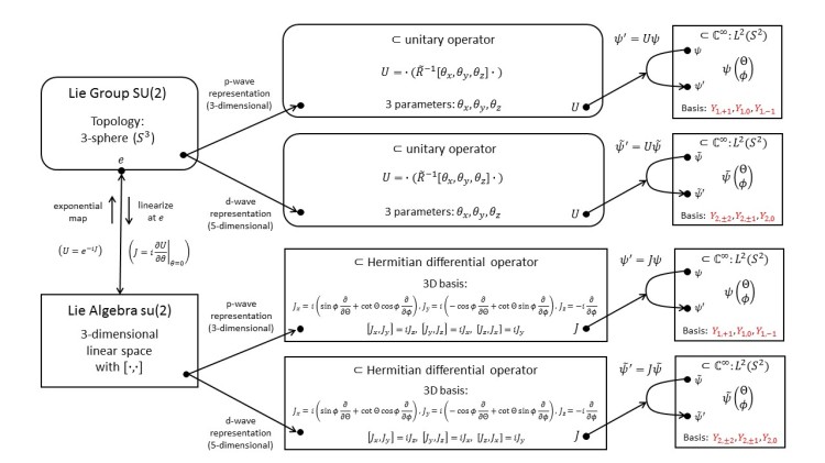
We find that the infinite-dimensional representation is reducible: it breaks up into the finite-dimensional representations we are already familiar with. Now we can understand the angular dependence of the electron orbitals (s, p, d, … waves) in atoms and why some of the energy levels are degenerated.
1.14 SU(2): Spinor-Field Representation; Two Types of Angular Momenta

We combine a scalar function and spinors into a new object: the spinor field. The SU(2) representation on spinor fields provides us with a deep insight into why there are two types of angular momenta: intrinsic angular momentum (or spin) and orbital angular momentum.
SU(2) and Tensors
1.15 SU(2): Tensor-Product Representation; Two Spin-1/2 Particles and Entanglement
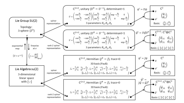
We switch gears and move on to another type of representation: the tensor-product representation. These representations are perfect for understanding multi-particle systems and quantum entanglement. We use rank-2 spinors to describe a system of two spin-1/2 particles.
1.16 SU(2): Tensor-Product Representation on 4D Vectors; Singlet and Triplet States

We “flatten” the rank-2 spinor into a 4D vector and find that this 4-dimensional representation is reducible. The states of definite combined spin form a basis that leads to the notion of singlet and triplet states. The singlet state has a maximum amount of entanglement and, when the two particles are separated and measured, exhibits “spooky action at a distance”.
1.17 SU(2): Representations on Symmetric and Antisymmetric Rank-2 Spinors
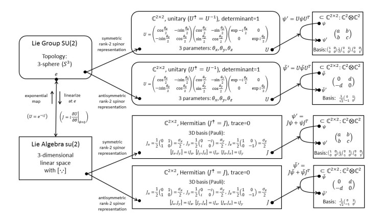
We let the tensor-product representation act on antisymmetric and symmetric rank-2 spinors. It turns out that these representations are just slightly disguised versions of the familiar 1- and 3-dimensional ones. To construct new representations from old ones, we can take the tensor product and decompose the result.
1.18 SU(2): Representation on Rank-3 Spinors; Index Notation

To describe a system of three spin-1/2 particles we need rank-3 spinors. How can we deal with these unwieldy objects? We introduce the index notation for tensors. Now we are good for any number of particles!
1.19 SU(2): Representation on Two-Particle Wave Functions

We take the tensor product of two wave functions. Now, we are able to describe two particles roaming through space. Interestingly, the resulting two-particle wave function is defined on a 6-dimensional configuration space, not our familiar 3D space, and quantum entanglement again adds a counter-intuitive twist to the story.
1.20 SU(2): Representations on (Anti)Symmetric Functions; Bosons and Fermions
We find that the representation on two-particle wave functions breaks up into one that is symmetric and one that is antisymmetric with respect to a particle exchange. These sub-representations describe systems of identical particles! Symmetric wave functions describe bosons and antisymmetric wave functions describe fermions. We discover that all fermions in the universe are entangled!
SO(3)
1.21 SO(3): The Group of Rotations in 3-Dimensional Euclidean Space

We move on to the group of rotations in 3-dimensional Euclidean space: SO(3). We explore the 3-dimensional (defining) representation and the 5-dimensional representation. Surprisingly, this group has only odd-dimensional representations! We compare the meaning of S in SO(3) to that in SU(2).
1.22 SO(3): Spinor Representations of the Algebra; Covering Group Spin(3)
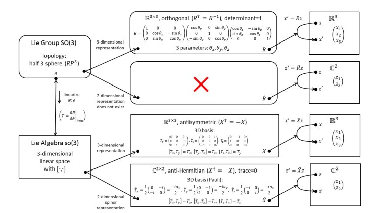
Does the Lie algebra so(3) also have only odd-dimensional representations? We learn about spinor representations. Taking the exponential map of a spinor representation takes us to the covering group. In the case of SO(3) this is Spin(3), which is isomorphic to our old friend SU(2)!
1.23 SO(3): Defining Representation with Axis-Angle Parameters; Group Topology

We examine the axis-angle parametrization of SO(3) and discover that this group has a rather strange topology! We discuss several ways to visualize this weird non-simply connected topology.
1.24 SO(3): Adjoint Representation

We construct the adjoint representation of SO(3). It turns out that the adjoint representation is equivalent to the defining representation!
1.25 SO(3): Defining Representation with Vectors as Generators; Cross Product
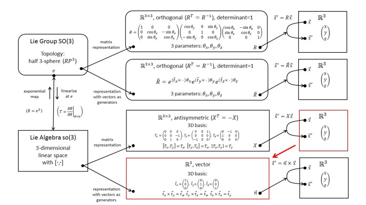
Instead of representing the Lie-algebra elements of so(3) by matrices, we can also represent them by vectors. For this to work out, we need a new operation. We discover the good old cross product!
1.26 SO(3): Application to Classical Angular Momentum; Noether’s Theorem
We apply SO(3) to classical mechanics. With the help of Noether’s theorem, we find the angular momentum of a particle. We compare and contrast classical angular momentum with quantum-mechanical angular momentum.
SO(3) and Functions
1.27 SO(3): Infinite-Dimensional Representation on Phase-Space Functions

We describe a particle in phase space. The functions on phase space, which are the classical observables, furnish an infinite-dimensional representation of SO(3).
1.28 SO(3): Representation with Functions as Generators; Poisson Bracket
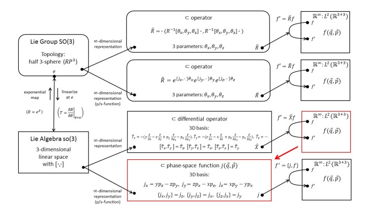
Instead of representing the Lie-algebra elements by differential operators, we can also represent them by phase-space functions. For this to work out, we need a new operation. We discover the Poisson bracket of classical Hamiltonian mechanics!
1.29 SO(3): Vector-Field Representation; Angular Momentum of Light

We apply SO(3) to the electromagnetic vector-potential field. With the help of Noether’s theorem, we find the angular momentum of light. The field’s vector character leads to two types of angular momenta: intrinsic (spin) and orbital.
SO(3) and Tensors
1.30 SO(3): Tensor-Product Representation; Decomposition

We take the tensor product of the defining representation of SO(3) with itself and find that it breaks up into three irreducible representations with dimensions five, three and one. To construct new representations from old ones, we can take the tensor product decompose the result.
Sp(1)
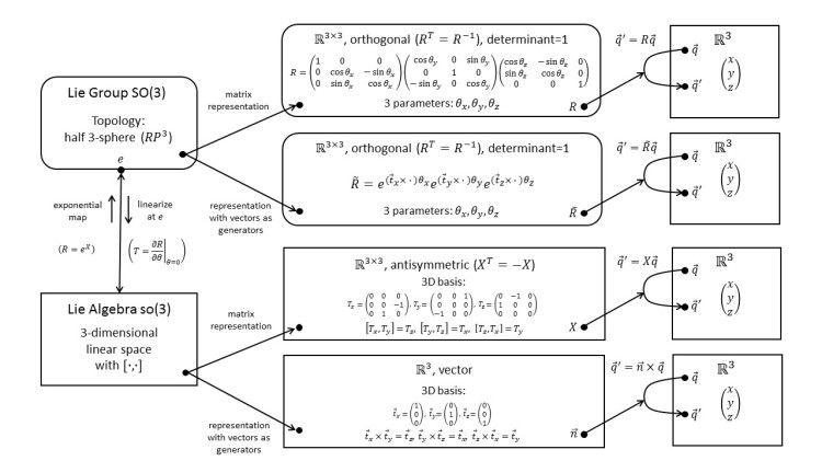
1.31 Sp(1): The Group of Quaternions of Unit Length

We explore the group of quaternions of unit length: Sp(1). Surprisingly, this group is isomorphic to SU(2)! Despite the abstract math, its adjoint representation has practical applications in computer graphics!
Reflection and Parity

2.1 D3: The Symmetry Group of the Equilateral Triangle; Semidirect Product
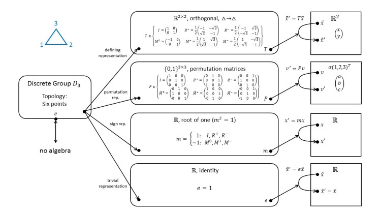
We take a break from Lie groups and look at some discrete groups. The symmetry group of the equilateral triangle, D3, has only six elements. We can represent them by 2D coordinate transformations or 3D vertex permutations. The group has a subgroup with reflection elements, Z2, and a subgroup with rotation elements, Z3. To reconstruct the full group from these two subgroups, we need the semidirect product.
2.2 Z2: The Cyclic Group of Order Two; Parity
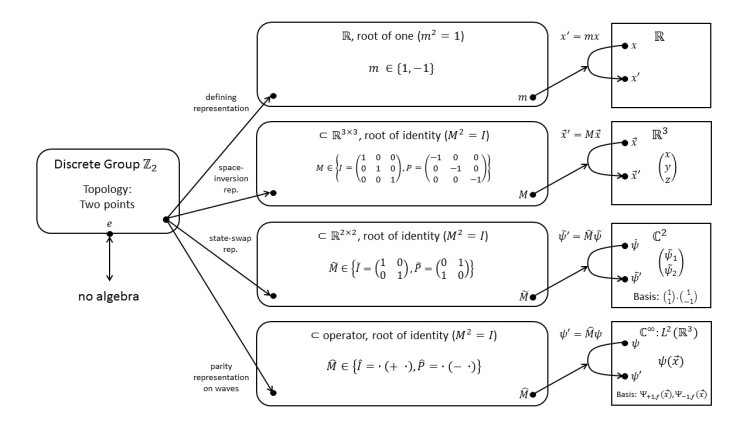
The cyclic group of order two, Z2, is the simplest, nontrivial, discrete group. It has many applications in physics: particle exchange, charge conjugation, time reversal, etc. Here, we focus on space inversion, a transformation that leads to the quantum observable known as parity.
Rotation in 4 Dimensions and Relativistic Space-Time

SO(4)
3.1 SO(4): The Group of Rotations in 4-Dimensional Euclidean Space
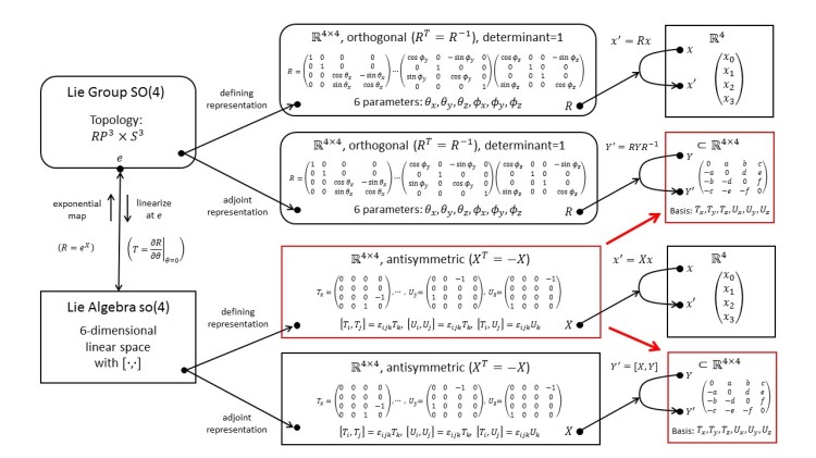
We move on to the group of rotations in 4-dimensional Euclidean space: SO(4). Examining this group will prepare us for the Lorentz group and special relativity. We explore the 4-dimensional defining representation and the 6-dimensional adjoint representation.
3.2 SO(4): Symmetric and Antisymmetric Tensor Representations

We construct the 16-dimensional tensor-product representation and find that it breaks up into a 10-dimensional symmetric and a 6-dimensional antisymmetric representation. Can the antisymmetric representation be broken up further?
3.3 SO(4): Self-Dual and Anti-Self-Dual Tensor Representations

Unlike for SO(3), the antisymmetric tensor representation of SO(4) can be broken up into two 3-dimensional representations: the self-dual and anti-self-dual representations! The Hodge dual is key to the construction of these representations.
3.4 SO(4): Self-Dual and Anti-Self-Dual Representations on 3D Vectors
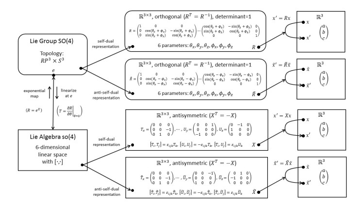
Rewriting the self-dual and anti-self-dual representations to act on 3D vectors shows that they are closely related to 3D rotation.
Spin(4)
3.5 Spin(4): Double Cover of SO(4); so(4)=so(3)+so(3)

We are switching from plane-rotation parameters to (anti-)self-dual double-rotation parameters. This takes us to Spin(4), the double cover of SO(4). Conveniently, this group breaks up into two copies of SU(2), which we already understand well.
3.6 Spin(4): The (0, 0), (1, 0), and (0, 1) Representations

We can enumerate all irreducible representations of Spin(4) by specifying two irreducible representations of SU(2): (j1, j2). Here we look at some representations that can be constructed from the spin-0 and spin-1 representations of SU(2).
3.7 Spin(4): The (1/2, 0), and (0, 1/2) Representations

We construct 2-dimensional spinor representations of Spin(4) by combining the spin-0 and spin-1/2 representations of SU(2). Interestingly, Spin(4) has two inequivalent 2-dimensional representations!
3.8 Spin(4): The (1, 1) Representation; Tensor Product (1, 0)x(0, 1)

We construct a 9-dimensional representation of Spin(4) from two copies of the spin-1 representation of SU(2) by taking the tensor product (1, 0)x(0, 1).
3.9 Spin(4): The (1/2, 1/2) Representation; 4D Rotation with Two SU(2) Matrices

We construct a 4-dimensional representation of Spin(4) from two copies of the spin-1/2 representation of SU(2). Amazingly, this representation on rank-2 spinors is equivalent to the (complexified) defining representation of Spin(4)! This means that we can rotate a 4D vector by acting on it with two SU(2) matrices.
3.10 Spin(4): The (1/2, 1/2) Representation; 4D Rotation with Two Quaternions

Given that Sp(1) is isomorphic to SU(2), we can do the same construction with unit quaternions! Now we can rotate a 4D vector by acting on it with two unit quaternions.
SO+(1,3)
3.11 SO+(1,3): The Group of Proper Orthochronous Lorentz Transformations

Moving on to space-time, we replace the Euclidean metric by the Minkowski metric. The group that preserves the Minkowski metric is the Lorentz group O(1,3). The proper orthochronous Lorentz group SO+(1,3) is the identity component of the Lorentz group. We examine the defining representation which acts on four vectors.
3.12 SO+(1,3): Dual Representation; Vectors and Covectors
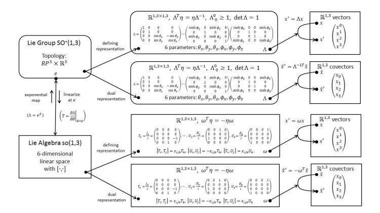
In contrast to SO(4), we find that under SO+(1,3) vectors and covectors transform differently. We introduce a notation with upstairs and downstairs indices to distinguish these two objects.
3.13 SO+(1,3): Space-Inverted and Time-Reversed Representations; Parity

The representation acting on space-inverted (= parity-inverted) vectors has the same generators of rotation but the generators of boost have the opposite sign. The same is true for the representation acting on time-reversed vectors.
SO+(1,3) and Fields
3.14 SO+(1,3): Scalar-Field Representation

We construct an infinite-dimensional representation that acts on scalar functions of space-time known as scalar fields.
3.15 SO+(1,3): Application to Scalar-Field Dynamics; Klein-Gordon Lagrangian

The requirement that the action of the scalar field must be Lorentz invariant leads us to the Klein-Gordon Lagrangian density, which describes the dynamics of a scalar field.
3.16 SO+(1,3): Vector-Field Representation

We construct an infinite-dimensional representation that acts on 4-vector fields. Now, the generators have two parts: one concerning the 4-vector structure and one concerning the space-time structure.
3.17 SO+(1,3): Application to Vector-Field Dynamics; Proca and Maxwell Lagrangians
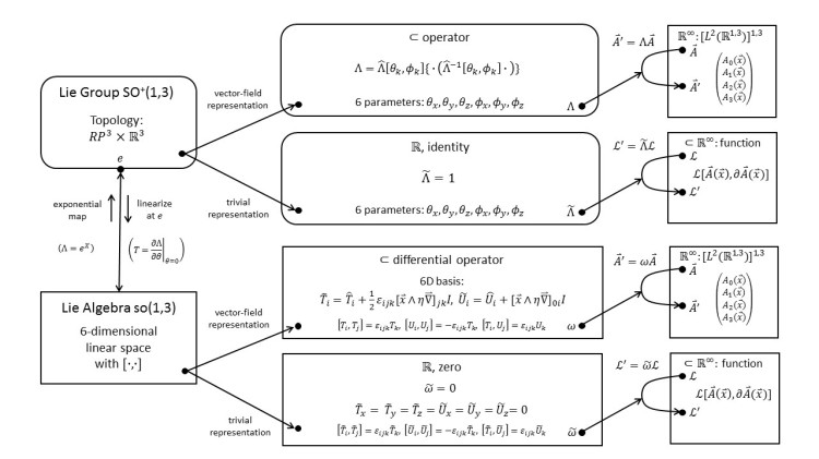
The requirement that the action of the 4-vector field must be Lorentz invariant leads us to the Proca Lagrangian density and the free Maxwell Lagrangian density.
SO+(1,3) and Tensors
3.18 SO+(1,3): Tensor-Product Representations; Decomposition
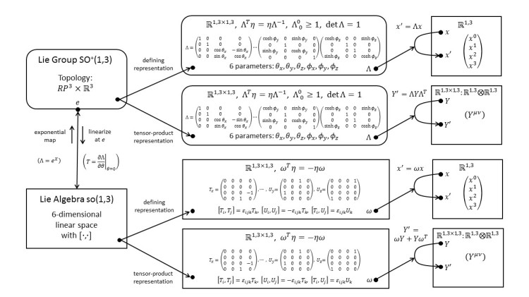
We construct the 16-dimensional tensor-product representation. The main difference to SO(4) is that the tensor now comes in four flavors. We illustrate this representation with the antisymmetric electromagnetic field-strength tensor and the symmetric energy-momentum tensor.
3.19 SO+(1,3): Self-Dual and Anti-Self-Dual Tensor Representations

Like for SO(4), the antisymmetric tensor representation of SO+(1,3) can be broken up into a self-dual and an anti-self-dual representations. In contrast to SO(4), the matrices of these two representations are now complex.
3.20 SO+(1,3): Self-Dual and Anti-Self-Dual Representations on 3D Vectors
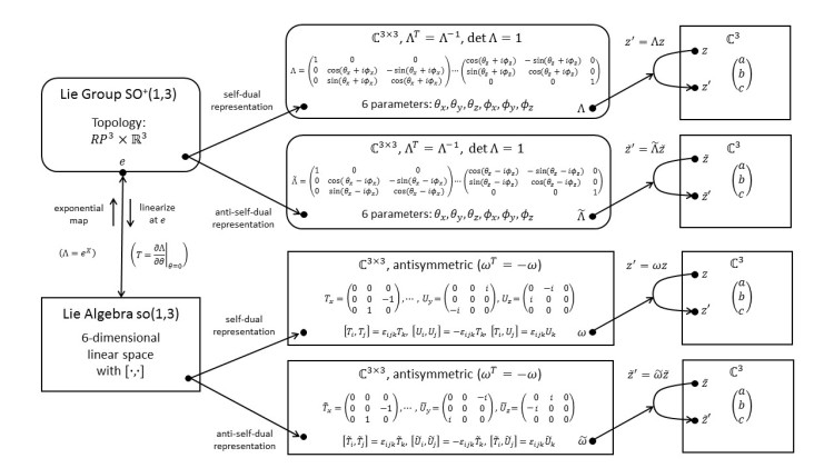
Rewriting the self-dual and anti-self-dual representations to act on 3D vectors reveals that they are complexified 3D rotations acting on complex 3D vectors.
Spin+(1,3)
3.21 Spin+(1,3): The Double Cover of SO+(1,3); so(1,3)C = so(3)C + so(3)C

Changing the transformation parameters takes us from SO+(1,3) to its double cover: Spin+(1,3). Unlike Spin(4), this group does not break up into two parts. But its complexification Spin+(1,3)C does break up into two copies of SU(2)C.
SL(2,C)
3.22 SL(2,C) = Spin+(1,3): The Relativistic Spin Group; Spinor Representations
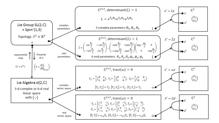
We study the group of complex 2×2 matrices with determinant one, SL(2,C). Amazingly, this group is isomorphic to Spin+(1,3)! We use the 2-dimensional (defining) representation to boost spinors.
3.23 SL(2,C): Left- and Right-Chiral Weyl-Spinor Representations; (1/2, 0) and (0, 1/2)

SL(2,C) has not only one but two inequivalent 2-dimensional representations. These representations are are related by parity inversion and known as the left- and right-chiral Weyl-spinor representations.
3.24 SL(2,C): Dirac-Spinor Representation; (1/2, 0) + (0, 1/2)
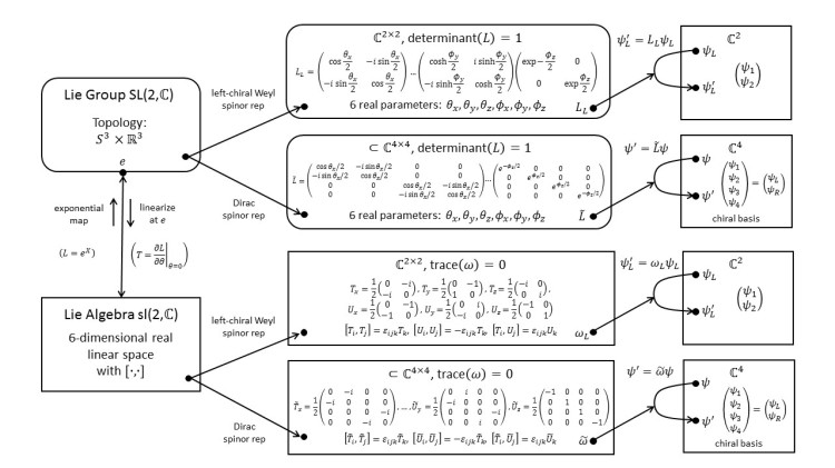
Taking the direct sum of the left- and right-chiral Weyl-spinor representations leads us to the Dirac-spinor representation, which respects parity.
3.25 SL(2,C): Dirac-Spinor Representations in the Chiral and Mass Basis

Dirac spinors can be written in different bases. In the chiral basis, we stack two Weyl spinors on top of each other. In the mass basis, we stack the sum and difference of two Weyl spinors. The latter basis is more convenient to describe massive particles like electrons.
3.26 SL(2,C): Four-Vector Representation; (1/2, 1/2) = (1/2, 0) x (0, 1/2)

We construct a 4-dimensional representation by taking the tensor product of the two 2-dimensional Weyl-spinor representations. Amazingly, this representation on rank-2 spinors is equivalent to the (complexified) defining representation of SO+(1,3)! This means that we can Lorentz transform a four vector by acting on it with an SL(2,C) matrix.
SL(2,C) and Fields
3.27 SL(2,C): Spinor-Field Representation

We construct an infinite-dimensional representation that acts on Dirac-spinor fields. Like for the representation on 4-vector fields, the generators have two parts: one concerning the Dirac spinors and one concerning the space-time structure, which is always the same.
3.28 SL(2,C): Application to Spinor-Field Dynamics; Dirac Lagrangian
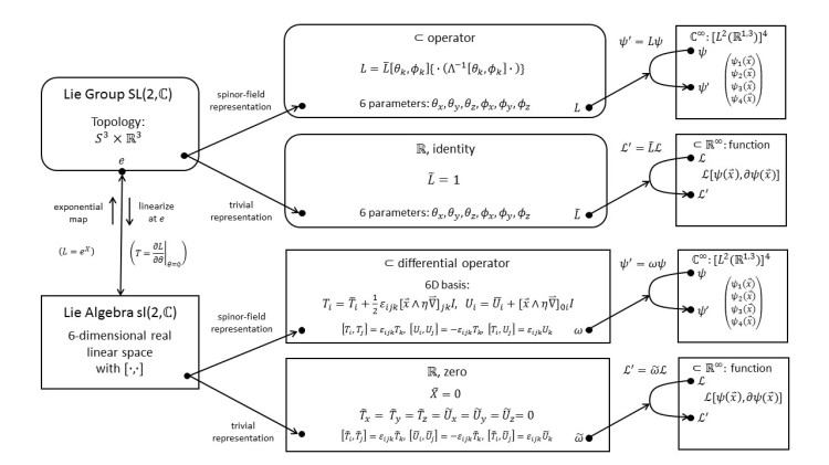
The requirement that the action of the Dirac-spinor field must be Lorentz invariant leads us to the Dirac Lagrangian density and the Weyl Lagrangian densities.
Rotation in 2 Dimensions and Electromagnetism

U(1)
4.1 U(1): The Group of Complex Numbers of Unit Length

We move on to the important group of complex numbers of unit length: U(1). This group has the topology of a circle and thus is also known as the circle group. Rather uncharacteristically for a Lie group, all its elements commute. U(1) has infinitely many irreducible representations, which can be labeled by integers.
4.2 U(1): Dual, Complex-Conjugate, Adjoint, and Product Representations
We discuss dual representations and complex-conjugate representations of U(1), which turn out to be the same thing. Then, we examine the adjoint representation, which turns out to be the trivial representation, and product representations.
4.3 U(1): Representation on Real 2-Dimensional Vectors
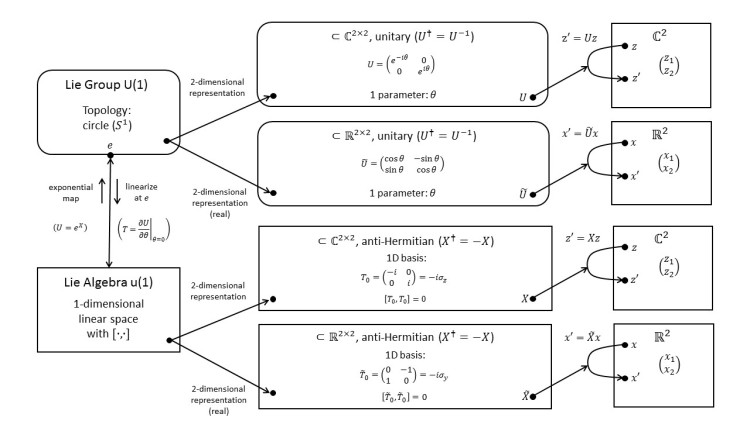
We construct a 2-dimensional representation that acts on real vectors. What does this new representation of U(1) describe? Rotations of ordinary 2D vectors!
4.4 U(1): Application to Photon Spin and Polarization

We use U(1) to describe quantum-mechanical spin along a particular direction in space. For massless particles, such as photons, the spin along their direction of motion is known as helicity, which is closely related to circular polarization.
U(1) and Functions
4.5 U(1): Infinite-Dimensional Representations; Circular Harmonics

We construct infinite-dimensional representations by letting U(1) act on functions of two real variables. Now, the Lie-algebra elements are differential operators and their eigenfunctions are the circular harmonics.
4.6 U(1): Application to Fourier Series and Fourier Coefficients

Using the basis from the previous example, we “unpack” the functions in the representation space. This leads us to a new representation of U(1) that acts on infinite-dimensional vectors, namely the Fourier coefficients of the functions.
U(1) and Gauge Fields
4.7 U(1): Application to the Electron Field; Electric Charge

We let U(1) act on the electron field, that is, the classical field, which when quantized yields electrons and positrons. This field is symmetric under U(1): it doesn’t matter what phase we call zero. The corresponding conserved quantity is the electric charge!
4.8 U(1): Local Gauge Transformations of the Electron Field; Fiber Bundles

The absolute phase of an electron field has no significance, but what about the difference between two phase values at two different events? Surprisingly, this difference is path dependent! To describe this effect mathematically, we introduce the idea of a fiber bundle and the associated connection field. This powerful and flexible description comes along with a new symmetry: local U(1) gauge symmetry.
4.9 U(1): Application to the Electromagnetic Potential; Covariant Derivative

We study the connection field and the closely related covariant derivative and how they are affected by local U(1) gauge transformations. Then, we discover that the connection field corresponds directly to the electromagnetic potential, which, in this context, is also known as a gauge field!
4.10 U(1): Application to the Electromagnetic Field Strength; Curvature

To locally characterize the path dependence of the electron field, we look at the phase mismatch along small loops in space-time. We learn about the curvature of fiber bundles and how it is affected by local U(1) gauge transformations. Then, we discover that the curvature corresponds directly to the electromagnetic field strength!
4.11 U(1): Application to Electromagnetic Interactions; Lagrangian of QED

The laws of physics cannot depend on our choice of coordinates. Thus, the action of quantum electrodynamics (QED) must remain invariant under local U(1) gauge transformations. Amazingly, this constraint is essentially enough to derive Maxwell’s equations and the Lorentz force law.
SO(2)
4.12 SO(2): The Group of Rotations in 2-Dimensional Euclidean Space; SO(2)=U(1)

We move on to the group of rotations in 2-dimensional Euclidean space: SO(2). This group turns out to be isomorphic to U(1). We explore the 2-dimensional or defining representation. Is this representation reducible or not?
4.13 SO(2): Spinor Representations; Spin(2)=SO(2)

We find that SO(2) has two inequivalent 1-dimensional spinor representations. These are the irreducible representations of SO(2)!
Rotation in Field Spaces and Nuclear Forces

5.1 To be written…

Appendices
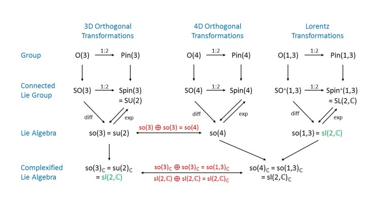
A.1 Low-Dimensional Lie Groups and their Relationships

The orthogonal groups preserve the Euclidean inner product, the unitary groups preserve the Hermitian inner product, and the symplectic groups preserve the quaternionic inner product. We explore some important relationships between these groups.

A.2 The Ladder Trick; Raising and Lowering Operators

SO(3), SU(2), and Sp(1) all have the same Lie algebra. The ladder trick, which makes use of raising and lowering operators, enables us to find all the representations of this algebra!
A.3 Symmetry and Conservation in Quantum Mechanics
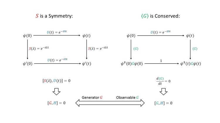
In quantum mechanics, observables are represented by operators. These operators are generators of transformations and thus there is a natural connection between observables and transformations. If the transformation is a symmetry (leaves the law of time evolution unaffected) then the observable is conserved (is time independent)!
A.4 Symmetry and Conservation in Classical Lagrangian Mechanics

In classical Lagrangian mechanics the relationship between symmetry and conservation is not as direct as in quantum mechanics. We discuss Noether’s theorem for particle theories that are symmetric with respect to rotation-like transformations.
A.5 Symmetry and Conservation in Classical Hamiltonian Mechanics

In classical Hamiltonian mechanics the relationship between symmetry and conservation is closer to that in quantum mechanics. The Poisson bracket of Hamiltonian mechanics takes on the role of the commutator bracket of quantum mechanics.
A.6 Noether’s Theorem for Particle Theories

We discuss Noether’s theorem for particle theories that are symmetric with respect to space translations, linear point transformations (e.g. rotations), and time translations. For each symmetry we obtain a conserved quantity.
A.7 Noether’s Theorem for Field Theories; Internal Symmetries

We discuss Noether’s theorem for field theories that are symmetric with respect to global field shifts and global linear field transformations. For each symmetry we obtain a locally conserved current from which we can derive a globally conserved quantity.
A.8 Noether’s Theorem for Field Theories; Space-Time Symmetries

We discuss Noether’s theorem for field theories that are symmetric with respect to global space-time translations and global Lorentz transformations. For each symmetry we obtain a locally conserved current from which we can derive a globally conserved quantity.
A.9 The Exterior Product; Area and Volume Elements
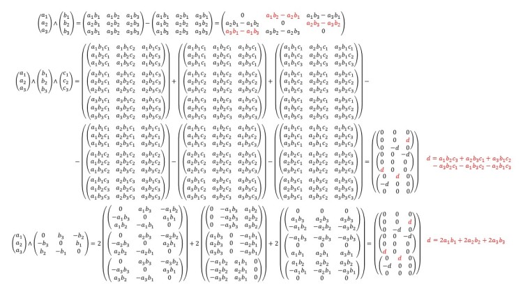
The exterior product generalizes the cross product and the triple product from 3- to higher-dimensional spaces. The exterior product can be visualized as an area or volume element.
A.10 The Hodge Dual in Euclidean Space

We examine totally antisymmetric tensors of increasing rank in two, three, and four dimensions. This reveals an interesting pattern that leads us to the idea of the Hodge dual.
A.11 The Exterior Derivative in 3D Euclidean Space; Gradient, Curl, and Divergence
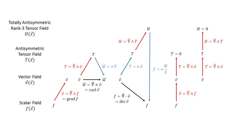
The exterior derivative and the Hodge dual are the tools that permit us to generalize and unify the gradient, curl, and divergence operators. In particular, we can generalize the curl operator from 3- to higher-dimensional spaces.
A.12 Euclid, Galileo, Einstein: Distance in Space and Time

We compare distance in space to “distance” in space-time according to Galileo and Einstein. This provides us with a way to visualize time dilation in the special theory of relativity.
A.13 Time Dilation, Lorentz Contraction, and Rest Energy

Starting from the Lorentz transformation, we study the effects of time dilation and Lorentz contraction. By regarding kinetic energy as rest-energy dilation, we can derive the rest-energy formula E=mc2.
A.14 From Rotation to Lorentz Transformation; Complexification
We explore relationships between rotation (in 3D and 4D Euclidean space) and Lorentz transformation (in space-time). Lie algebras and their complexification play a crucial role.
A.15 The Irreducible Representations of the Lorentz Group
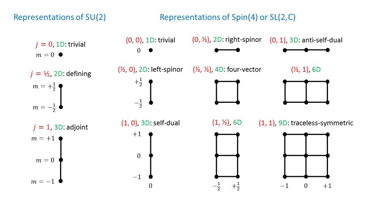
We look at the weight diagrams of important representations of the (double cover of the) Lorentz group and compare them to the representations of SU(2).
A.16 Decoding the Klein-Gordon Equation

The Klein-Gordon equation describes a scalar field that satisfies the symmetries of special relativity. The equation is presented in various forms and notations.
A.17 Decoding the Dirac Equation
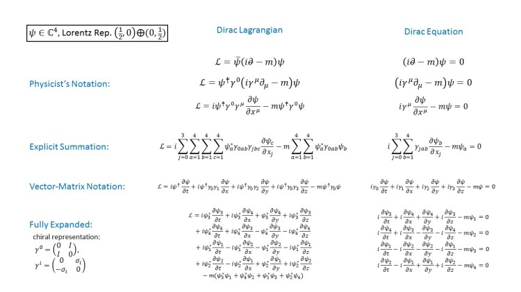
The Dirac equation describes a spinor field, such as the electron/positron field, that satisfies the symmetries of special relativity. The equation is presented in various forms and notations.
A.18 Decoding the Proca and Free Maxwell Equation

The Proca equation describes a vector field that satisfies the symmetries of special relativity. The free Maxwell equation is the same for a dispersion-free (= massless) vector field, such as the electromagnetic potential field (or photon field). The equations are presented in various forms and notations.
A.19 Metric, Connection, and Curvature in 2D Riemannian Geometry

We compare the metric, connection, and curvature of a 2D Euclidean space with Cartesian coordinates, a 2D Euclidean space with polar coordinates, and a 2D spherical space with spherical coordinates.
A.20 Christoffel Symbols for Polar Coordinates

We use an intuitive geometric method to determine the Christoffel symbols for a 2D Euclidean space with polar coordinates.
A.21 From Lorentz and Gauge Symmetry to Maxwell’s Equations

We sketch the logical steps that lead from Lorentz symmetry and U(1) gauge symmetry to Maxwell’s equations of electrodynamics.
